Leverage effect could bring seasonal Q1 stock market drawdown
The recent Q4 volatility patterns of the major U.S stock market Index, such as Dow Jones Industrial Average, S&P500, Nasdaq100 and Russell 3000 could have been a forthcoming market signal of a volatility build-up going into Q1 2025, as among the seasonal factors determining a wider stock market correction. In the past weeks, stock markets have factored in some hard macroeconomic data and idiosyncratic volatility market moves which all point to the possible direction of a momentum build-up into a seasonal Q1 2025 stock market correction, meanwhile, assets managers across the financial industry could have been anticipating a profit taking momentum, derived by the forthcoming passage of duties in the Oval Office, and with that, all raft of changes in economic and fiscal policy could inevitably require wider macroeconomic adjustments and financial assets adjustments.
Setting apart, what should be exogenous factors to stock market prices, the recent stock market volatility seems to hint at higher volatility momentum build-up also in the large stock market Index as DJIA, S&P500, NDX, Russell3000, and that with some discrete probability a correction in Q1 2025 could be in the realm of concrete seasonal outcomes for the stock market and financial assets broadly. In this instance, because most people tend to want to know how large could be the Q1 stock market correction, here anybody can find the data based on historical Q1 drawdown patterns:
Aggregate Q1 2025 Drawdown Estimates for DJIA: Historical Q1 Drawdown: -15.23%, Adjusted Q1 Drawdown: -12.45%.
Aggregate Q1 2025 Drawdown Estimates for S&P500: Historical Q1 Drawdown: -18.67%, Adjusted Q1 Drawdown: -14.89%.
Aggregate Q1 2025 Drawdown Estimates for NASDAQ100 :Historical Q1 Drawdown: -20.45%,
Adjusted Q1 Drawdown: -16.78%.
Aggregate Q1 2025 Drawdown Estimates for RUSSELL 3000: Historical Q1 Drawdown: -16.34%, Adjusted Q1 Drawdown: -13.12%.
To understand and forecast volatility patterns of these stock market indexes: DJIA, S&P500, NDX, and Russell3000, a thorough methodology of rolling standard deviation and econometrics quantitative models such as GARCH and EGARCH have been implemented together with ARIMA and SARIMA forecast. Indeed, accurate historical patterns of VaR 95,97.5,99,99.9 violation days have been inference from the 2007/2024 historical time-series, in order to determine the past quarters’ volatility patterns and to forecast the Q1 2025 possible seasonal drawdown scenario. DJIA(^DJI), S&P500(^GSPC), NDX(^NDX), Russell 3000(^RUA) time-series present the following results for 7day and 21day annualised volatility.

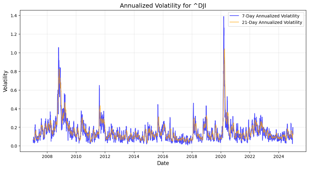
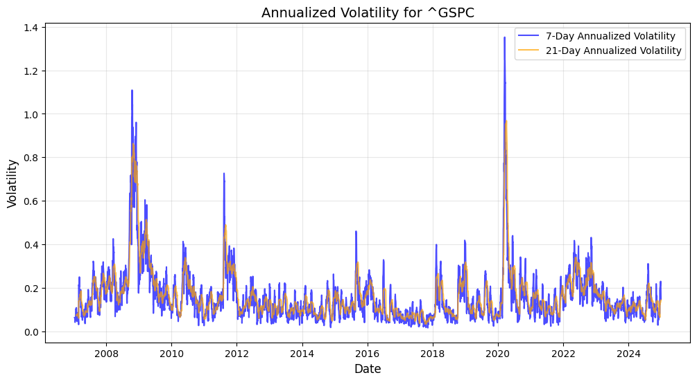
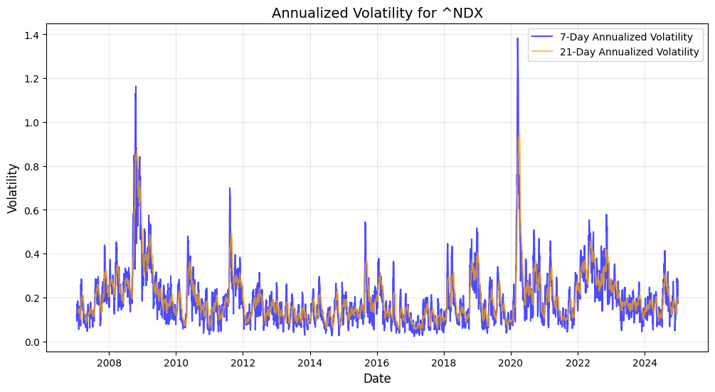
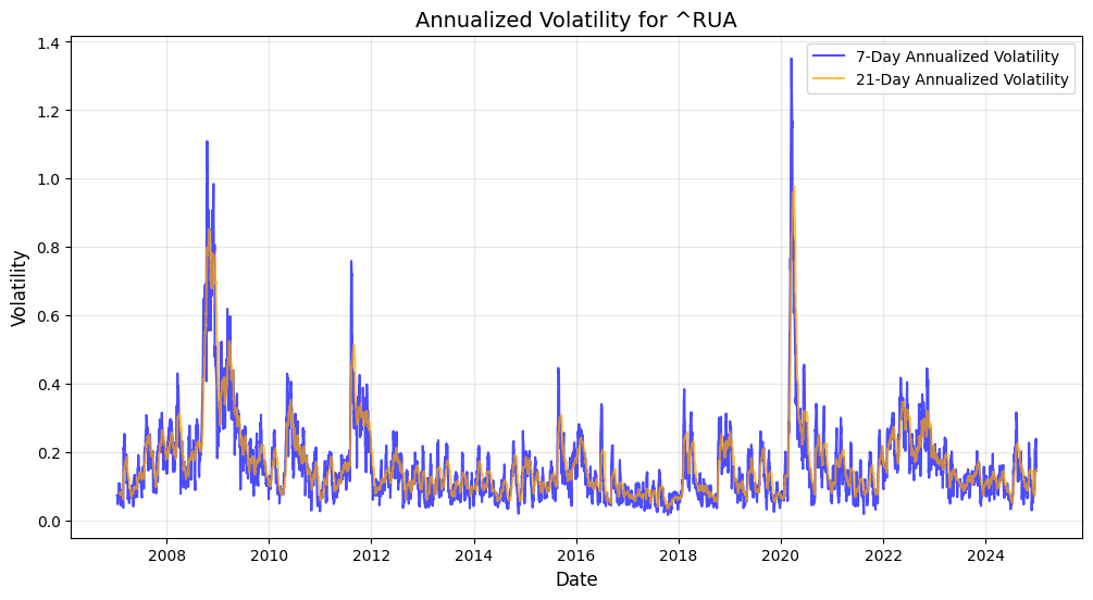
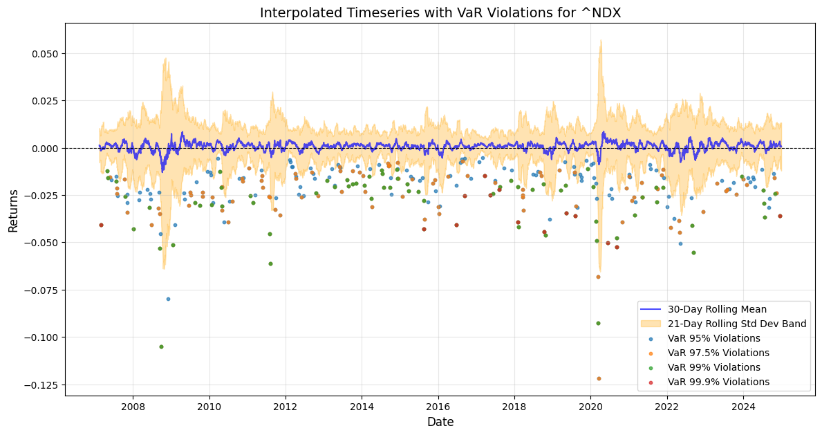
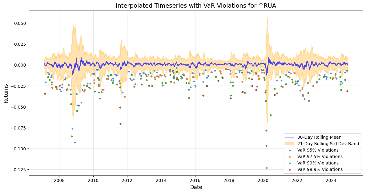
With the rolling 7day and 21day standard deviation annualised, the VaR violation days across the discrete time-series have been extracted for the following results VaR Violations Summary: VaR(95) DJIA(-2.08%) 285 days, S&P500 (-2.23%) 281 days, NDX (-2.5%) 285 days, Russell 3000 (-2.27%) 284 days, VaR(97.5) DJIA (-2.33%) 174 days, SPX (-2.42%) 177, NDX (-2.78%) 169, RUA (-2.48%) 178, for VaR(99) DJIA (-2.58%) 89 days, SPX (-2.71%) 102 days, NDX (-3.18%) 88 days, RUA (-2.71%) 100 days, last but not least VaR(99.9) DJIA (-2.85%) 18 days, SPX (-2.85%) 18 days, NDX (-3.77%) 15 days, RUA (-3.04%) 18 days.
In the below charts the 21-day rolling standard deviation band has been pulled with the 30-day rolling mean returns, and the coloured dots are the integrated VaR violation days across the discrete time-series, from where it can be appreciated that Q3 Q4 2024 periods do exhibit relative clustering of VaR 99% and VaR 99.9% days in this latter part of the year as a consistent high one-day volatility pattern that could be building stock market drawdown momentum. What can also be defined as Kairos καιρός the critical momentum of time opportunity for the Q1 2025 seasonal stock market correction?
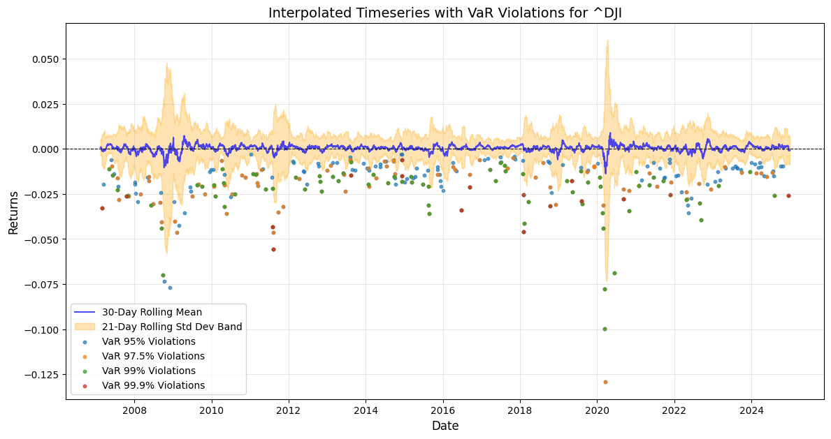
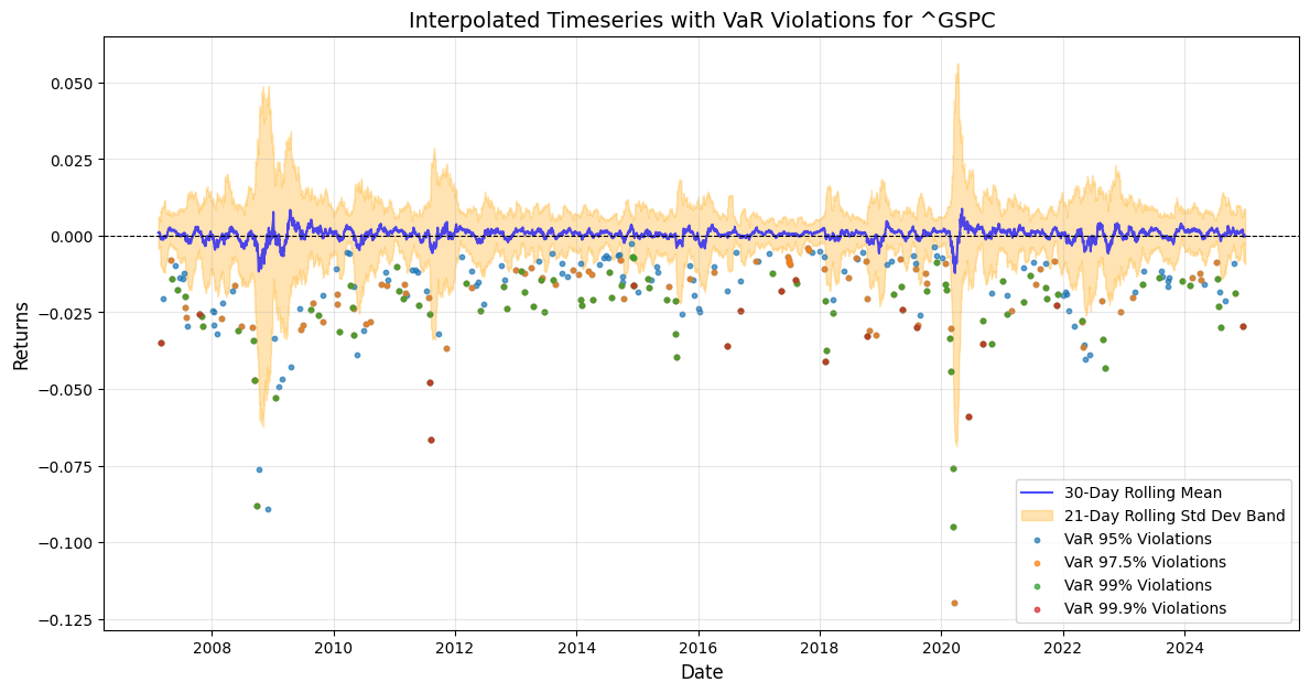
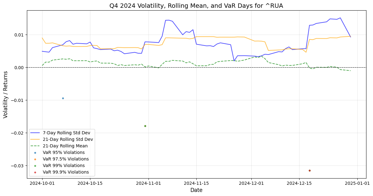
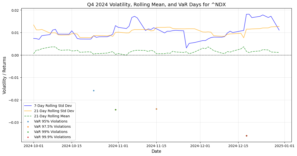
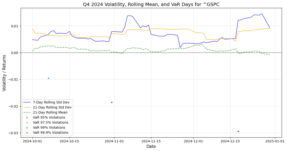
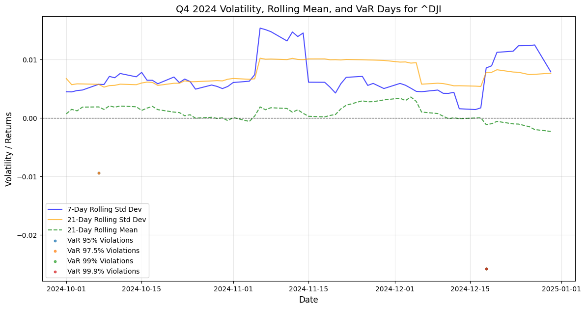
In these charts, the methodology follows through in narrowing down the discrete time-series window reaction function of volatility patterns of the stock market indexes extracting the Q3-Q4 rolling Volatility mean overlayed with VaR days violation for the same timeframe, the data have been refined to derive the ratio of VaR days violation occurred in Q4 in proportion to the whole 2024. Narrowing down the timeframe observation scope has provided these hard data for Q4: DJIA Var(95) 4 days violation as 18.75% occurrence proportion to 2024. S&P500 VaR(95) 3 days violations during Q4 equates to 21.4% of yearly S&P500 VaR(95) violations, Nasdaq100 VaR(95) 5 days violations in Q4 equating to 27.8% of yearly VaR(95), Russell 3000 VaR(95) 4 days violation in Q4 equating to 23.5% of yearly 2024 VaR(95). Then going forward with VaR(97.5): DJIA 1 day,16.67% of yearly data, S&P500 2 Days = 20% of yearly VaR(97.5), Nasdaq100 4 Days = 44,4% of yearly 2024 VaR(97.5) from here we can gather the fact that Nasdaq100 VaR(97.5) violations have been generated for 44,4% during Q4, while Russell 3000 2 days = 22,2% of yearly data. For VaR(99) DJIA 1 day = 50% of yearly occurrence in 2024, S&P500 2 days = 33,3% of yearly violations, Nasdaq100 2 days = 40% of yearly observations, Russell 3000 2 days = 33,3% of yearly VaR(99) episodes. Then the VaR(99,9) violation gives clear hard data, as for all indexes DJIA, S&P500, Nasdaq100 and Russell 3000, the only one VaR(99,9) data point has been generated in Q4 by stock markets, this also validates the findings that high volatility patterns have been gathering momentum in Q4 2024 and these should generate a Q1 stock market drawdown.
After narrowing down the timeframe to Q4 for VaR violations inference with rolling standard deviations then the implementation of the quantitative econometrics models as: GARCH(1,1), EGARCH(1,1) to calculate the indexes conditional volatility and time-varying volatility in financial markets, while EGARCH allows to gather the asymmetric effects of volatility shocks, while volatility decomposition methodology as been utilised to filter through noise in the price variance and volatility in order to gather another precise data for Q4 volatility patterns and VaR.
DJIA GARCH EGARCH results:
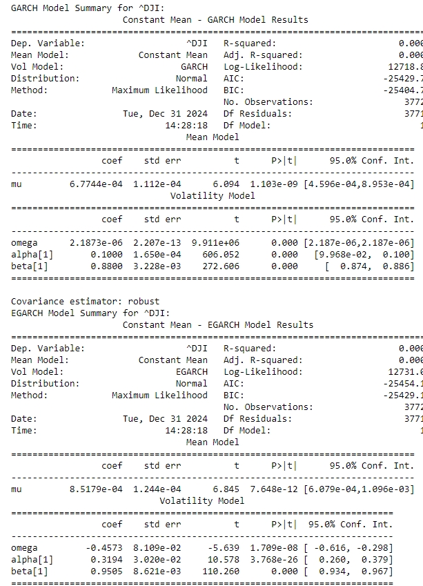

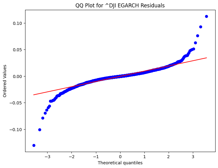
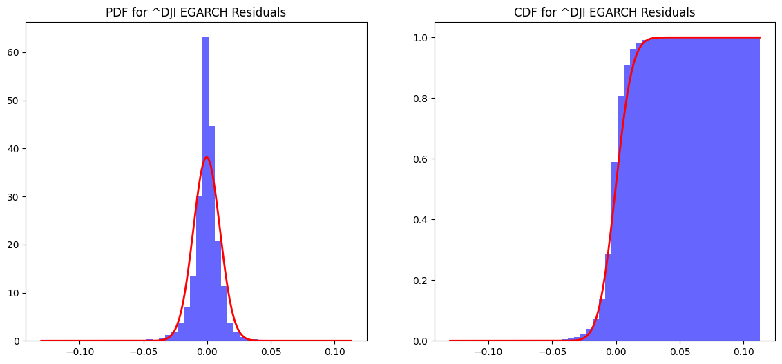
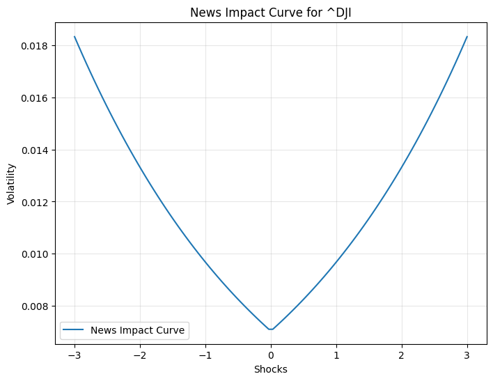
The GARCH model results show a significant impact of past volatility (alpha) and persistence (beta) on current volatility, with coefficients of 0.1000 and 0.8800, respectively. The EGARCH model, on the other hand, indicates a higher persistence (beta[1] = 0.9505) and a significant asymmetric effect (alpha[1] = 0.3194), suggesting that negative shocks have a more pronounced impact on volatility than positive ones. The log-likelihood values and information criteria (AIC and BIC) suggest that the EGARCH model provides a slightly better fit to the data compared to the GARCH model. These findings are crucial for understanding market behaviour and for risk management, as they highlight the importance of considering both the magnitude and direction of market shocks in volatility modelling. The GARCH residuals QQ plot shows some deviations from the theoretical quantiles, particularly in the tails, indicating that the residuals may not be perfectly normally distributed. Similarly, the EGARCH residuals QQ plot also exhibits deviations, suggesting that while the EGARCH model captures volatility clustering and asymmetry, it may not fully account for all distributional characteristics of the data. The model parameters for ^DJI, including the mean (mu), volatility intercept (omega), and coefficients for past shocks (alpha[1]) and persistence (beta[1]), highlight the dynamic nature of market volatility. The EGARCH model, with its higher persistence (beta[1] = 0.9505) and significant asymmetric effect (alpha[1] = 0.3194), underscores the importance of considering the direction of market shocks in volatility modelling. These findings are crucial for refining risk management strategies and improving the accuracy of financial forecasts. The News Impact Curve for the Dow Jones Industrial Average (^DJI) illustrates how different magnitudes of shocks influence volatility. The curve shows that both positive and negative shocks increase volatility, but the impact is asymmetric. Negative shocks tend to have a more pronounced effect on volatility compared to positive shocks of the same magnitude. This asymmetry is a key feature often captured by models like EGARCH, which accounts for the differential impact of market news. The Probability Density Function (PDF) for the GARCH residuals of ^DJI provides a visual representation of the distribution of these residuals. The PDF indicates that the residuals are centred around zero, which is expected if the model is well-specified. However, the presence of fat tails suggests that extreme values occur more frequently than would be expected under a normal distribution.
S&P500 GARCH, EGARCH results:
The GARCH model results indicate a significant impact of past volatility (alpha[1] = 0.1000) and high persistence (beta[1] = 0.8800) on current volatility. The mean return (mu) is estimated at 7.5394e-04, suggesting a positive average return over the period analyzed. The EGARCH model, which accounts for the asymmetric effects of shocks, shows a slightly higher mean return (mu = 9.1100e-04) and similar persistence (beta[1] = 0.9500). The alpha[1] coefficient in the EGARCH model (0.3176) indicates that negative shocks have a more pronounced impact on volatility than positive shocks, a common feature in financial markets.
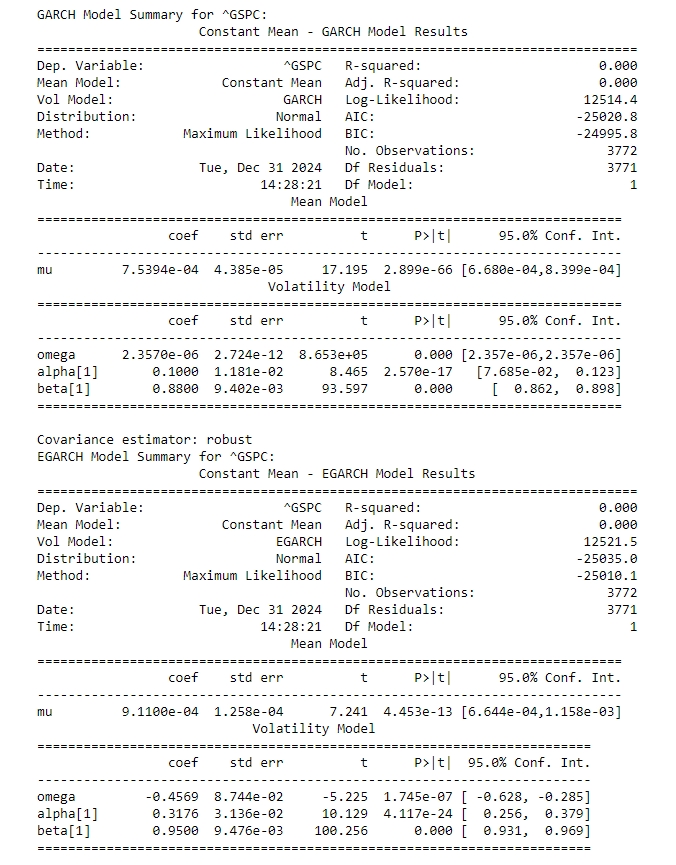

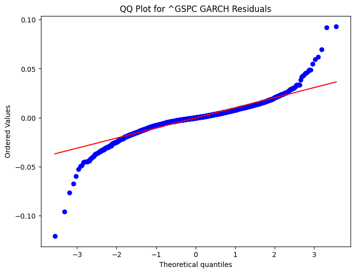
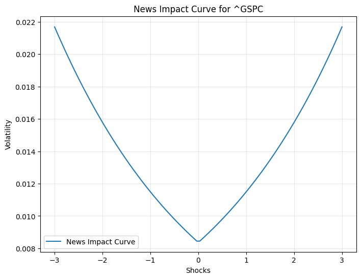
Both models have high log-likelihood values, with the EGARCH model providing a marginally better fit as indicated by the lower AIC and BIC values. The model parameters for ^GSPC, including the mean (mu = 0.000911), volatility intercept (omega = -0.456857), and coefficients for past shocks (alpha[1] = 0.317615) and persistence (beta[1] = 0.949978), highlight the dynamic nature of market volatility. The EGARCH model, with its high persistence and significant asymmetric effect, underscores the importance of considering the direction of market shocks in volatility modelling. The QQ plots for the residuals of the GARCH and EGARCH models applied to the S&P 500 (^GSPC) provide a visual assessment of the normality of the model errors. The GARCH residuals QQ plot shows some deviations from the theoretical quantiles, particularly in the tails, indicating that the residuals may not be perfectly normally distributed. Similarly, the EGARCH residuals QQ plot also exhibits deviations, suggesting that while the EGARCH model captures volatility clustering and asymmetry, it may not fully account for all distributional characteristics of the data. The News Impact Curve for ^GSPC illustrates the asymmetric effect of shocks on volatility, a phenomenon well-documented in financial markets. The curve indicates that negative shocks have a more pronounced impact on volatility compared to positive shocks of the same magnitude. This asymmetry is effectively captured by the EGARCH model, which incorporates a leverage effect to account for the differential impact of market news.
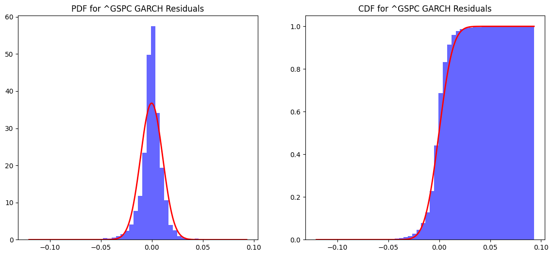
The Probability Density Function (PDF) and Cumulative Distribution Function (CDF) plots for the GARCH and EGARCH residuals offer insights into the distributional properties of the model errors. The PDFs reveal that the residuals are centred around zero, which is consistent with well-specified models. However, the presence of fat tails in both GARCH and EGARCH residuals suggests that extreme values occur more frequently than would be expected under a normal distribution.
NASDAQ 100 GARCH and EGARCH model summary:
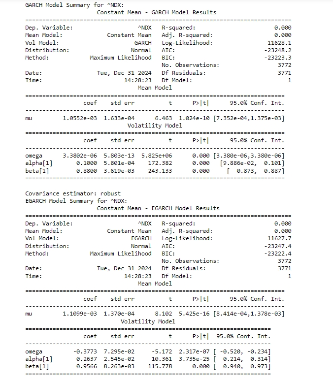

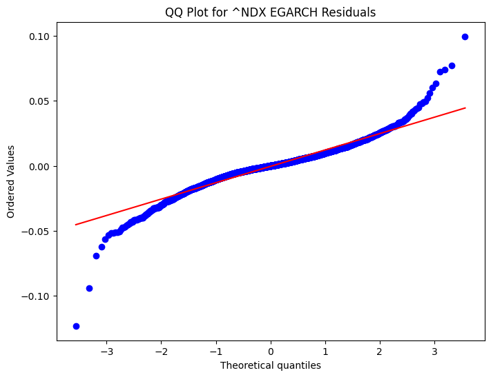
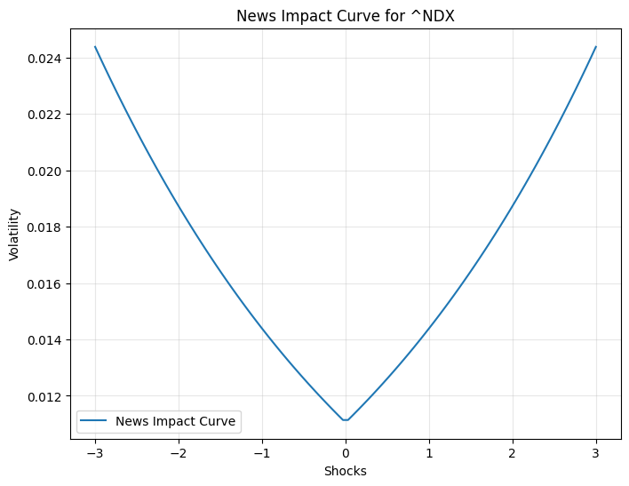

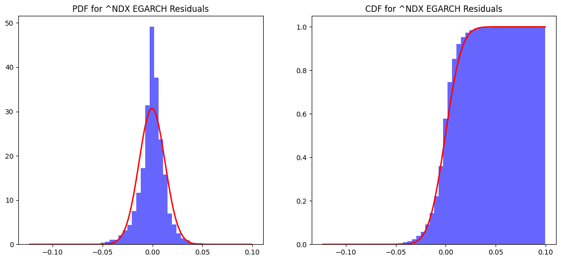
The summary for the Nasdaq 100 Index (^NDX) using GARCH and EGARCH models reveals key insights into its volatility dynamics. Both models indicate a positive and statistically significant average daily return, with the GARCH model estimating it at 0.001055 and the EGARCH model at 0.001109. Volatility persistence is high in both cases, with the GARCH model showing a beta of 0.880 and the EGARCH model a slightly higher beta of 0.956, suggesting that volatility shocks decay slowly over time. However, the EGARCH model highlights a stronger impact of past shocks on current volatility (alpha = 0.2637 vs. 0.1000 in GARCH) and captures the asymmetric effect of negative shocks, a feature absent in the GARCH model. While both models fit the data well, the EGARCH model’s marginally lower AIC makes it a slightly better choice, particularly when accounting for the leverage effect. These findings underscore the importance of model selection in understanding and forecasting market volatility. The QQ plots for the GARCH and EGARCH model residuals provide a visual assessment of how well the residuals conform to a normal distribution. In both plots, the ordered values of the residuals are plotted against theoretical quantiles of a normal distribution. For the GARCH model, the QQ plot shows some deviations from the straight line, particularly in the tails, indicating that the residuals may not perfectly follow a normal distribution. Similarly, the QQ plot for the EGARCH model also exhibits slight deviations in the tails, suggesting that while the model captures much of the volatility dynamics, there are still some extreme values that deviate from normality. These deviations highlight the presence of heavier tails in the residual distribution, which is a common characteristic in financial time series. Overall, the QQ plots suggest that while both models provide a good fit, there is room for further refinement to better capture the distributional properties of the residuals.The News Impact Curve illustrates how shocks (unexpected changes) affect the volatility of the Nasdaq Composite Index (~NDX). The curve is asymmetric, indicating that negative shocks (left side of the graph) have a more pronounced impact on volatility compared to positive shocks (right side). This asymmetry is consistent with the leverage effect, where negative news tends to increase market volatility more than positive news of the same magnitude. The Probability Density Function (PDF) for the GARCH model residuals shows the distribution of the residuals, which represent the differences between the observed and predicted values. The PDF is centred around zero, indicating that the residuals are symmetrically distributed. However, the tails of the distribution are slightly thicker than those of a normal distribution, suggesting the presence of extreme values or outliers. This is consistent with the QQ plot findings, where deviations in the tails were observed. The PDFs for both GARCH and EGARCH residuals show symmetric distributions, but the EGARCH model better captures extreme values with thinner tails. The CDF for EGARCH residuals confirms the symmetric and well-behaved nature of the distribution, supporting the model’s effectiveness in modelling volatility dynamics.
Russell 3000 GARCH and EGARCH model summary:
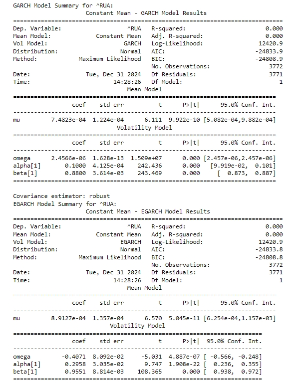
The mean return (mu) is estimated to be 7.4823e-04 (0.00074823), which is statistically significant (p-value < 0.05). This indicates a positive and significant average daily return for the Russell 3000 Index (^RUA). The baseline volatility is 2.4566e-06, which is very small but statistically significant. The coefficient for the ARCH term (lagged squared residuals) is 0.1000, indicating that past shocks have a moderate impact on current volatility. The coefficient for the GARCH term (lagged conditional variance) is 0.8800, suggesting high persistence in volatility. The sum of alpha and beta (0.1000 + 0.8800 = 0.9800) is close to 1, indicating that volatility shocks decay slowly and have a long-lasting effect.. Both models show high persistence in volatility (beta close to 1), but the EGARCH model has a slightly higher beta (0.9551 vs. 0.8800). The EGARCH model suggests a stronger impact of past shocks on current volatility (alpha = 0.2958 vs. 0.1000 in GARCH), the EGARCH model explicitly accounts for the asymmetric effect of shocks (negative shocks increase volatility more than positive shocks) reinforcing the Leverage Effect in markets. The AIC and BIC values are very close for both models, but the EGARCH model has a slightly lower AIC (-24833.8 vs. -24833.9), suggesting it might be a marginally better fit.
Q3 Q4 GARCH EGARCH models inference with Rolling Standard Deviation and VaR violations
The provided charts combine volatility measures and Value-at-Risk (VaR) violations for three major indices: the Dow Jones Industrial Average (DJI), the S&P 500 (~GSPC), and the Nasdaq Composite (~NDX) during the period from Q3 2024 to Q1 2025. These charts are useful for understanding the volatility dynamics and the performance of VaR models in capturing extreme market movements.
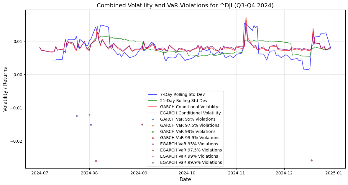
The chart includes 7-day rolling standard deviation, 21-day rolling standard deviation, GARCH conditional volatility, and EGARCH conditional volatility. Volatility shows fluctuations over time, with spikes indicating periods of increased market uncertainty. The GARCH and EGARCH conditional volatility measures tend to be smoother than the rolling standard deviations, reflecting the models’ ability to capture persistent volatility patterns. VaR violations are marked for both GARCH and EGARCH models at the 95%, 97.5%, 99%, and 99.9% confidence levels. Violations occur when actual returns exceed the VaR thresholds, indicating that the models underestimated the risk during those periods. The EGARCH model generally shows fewer violations compared to the GARCH model, suggesting it better captures extreme market movements, likely due to its ability to model asymmetric volatility (leverage effect).
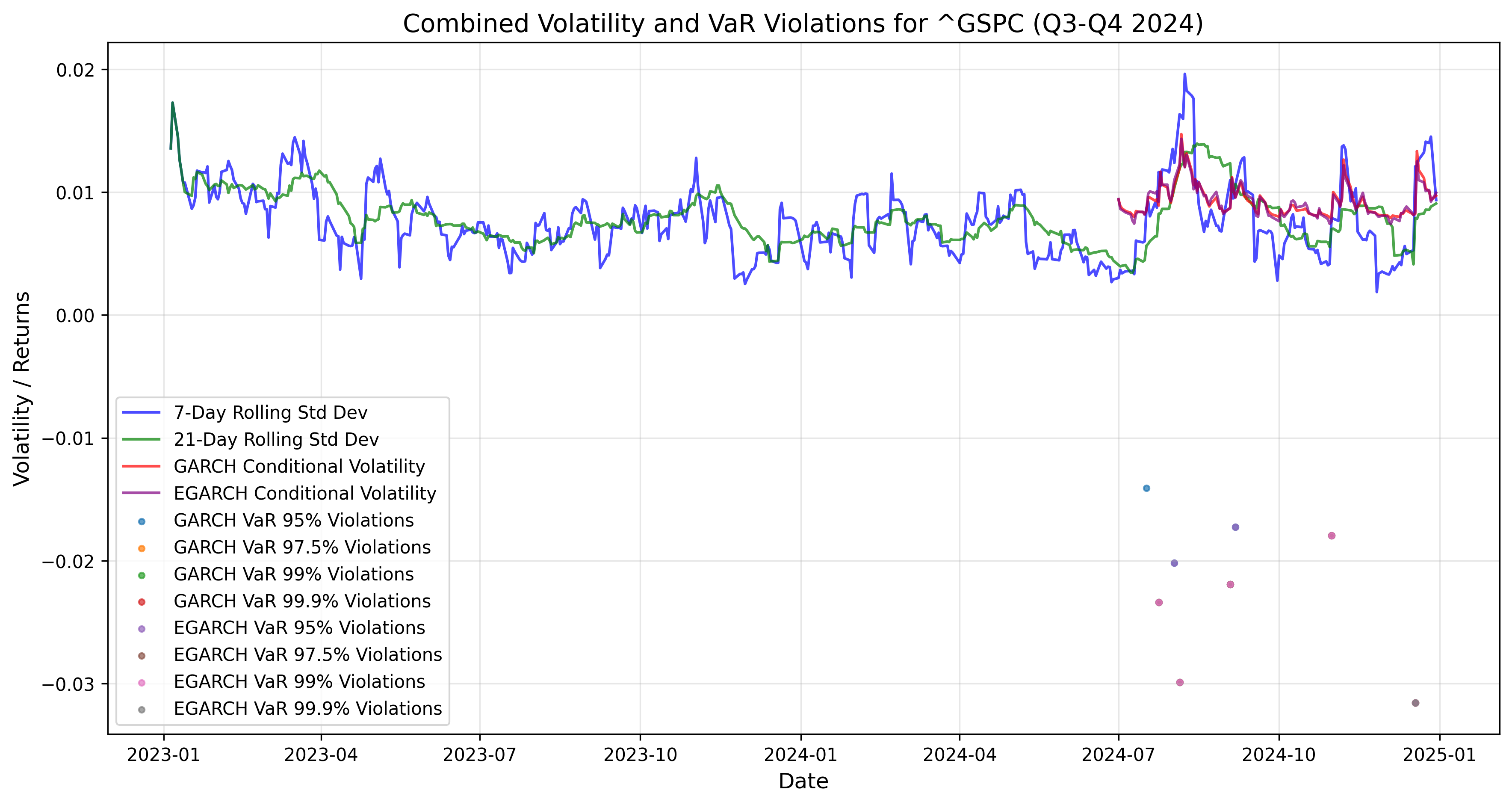
Similar to the DJI, the chart shows 7-day rolling standard deviation, 21-day rolling standard deviation, GARCH conditional volatility, and EGARCH conditional volatility. Volatility spikes are observed during periods of market stress, with the GARCH and EGARCH models providing smoother estimates of conditional volatility. VaR violations are marked for both GARCH and EGARCH models at various confidence levels. The EGARCH model again shows fewer violations compared to the GARCH model, indicating its superior performance in capturing extreme events. The frequency of violations increases at higher confidence levels (e.g., 99% and 99.9%), reflecting the difficulty of predicting extreme tail events.
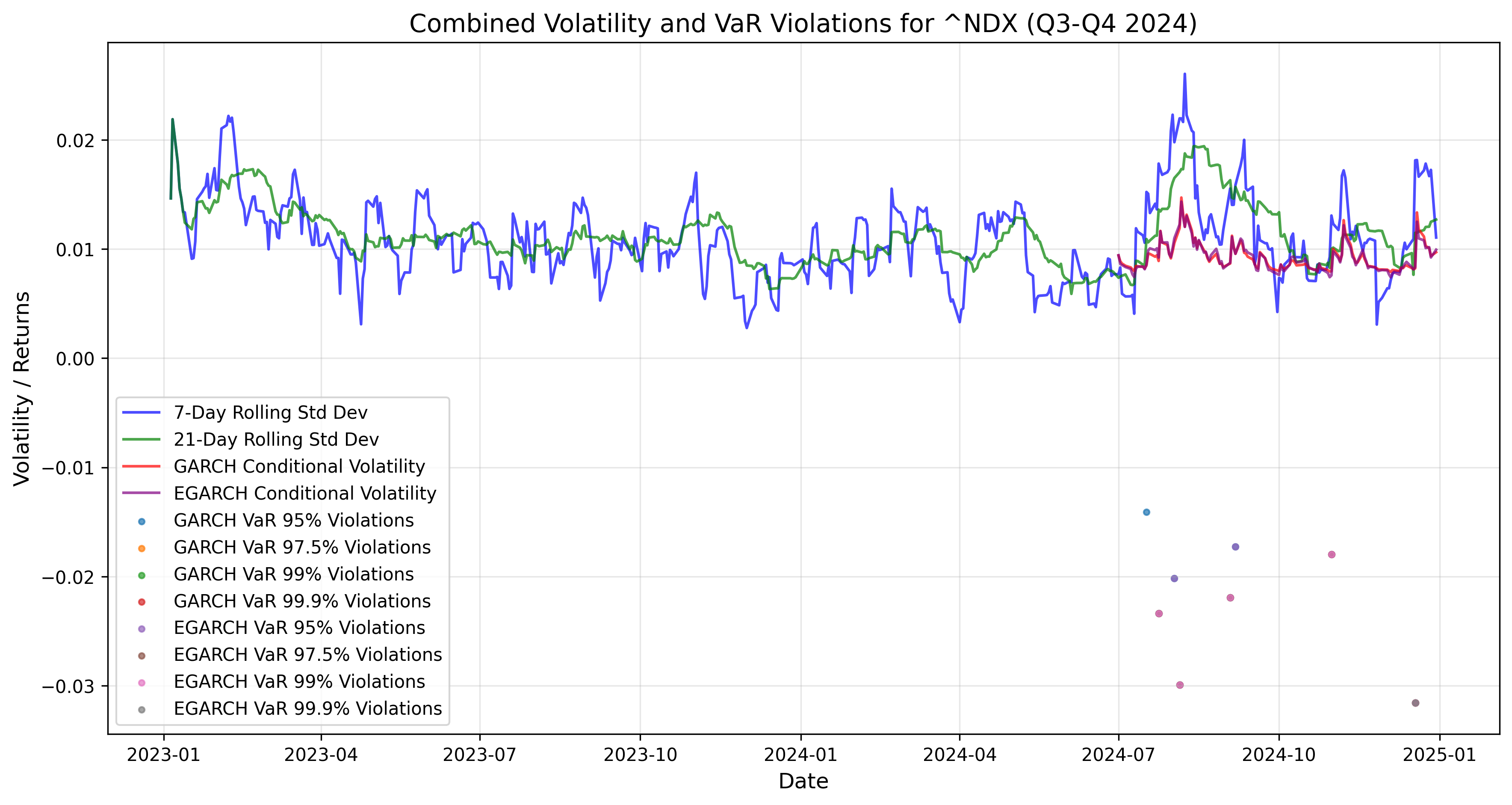
The chart includes the same volatility measures as the other indices: 7-day rolling standard deviation, 21-day rolling standard deviation, GARCH conditional volatility, and EGARCH conditional volatility. The ~NDX exhibits higher volatility compared to the DJI and S&P 500, consistent with the technology sector’s greater sensitivity to market movements. VaR violations are marked for both GARCH and EGARCH models at various confidence levels. The EGARCH model shows fewer violations than the GARCH model, particularly at higher confidence levels, highlighting its effectiveness in modelling the ~NDX’s volatility dynamics. The ~NDX’s higher volatility leads to more frequent VaR violations compared to the DJI and S&P 500, especially at extreme confidence levels (e.g., 99.9%).

This chart combines volatility measures and Value-at-Risk (VaR) violations for the Russell 3000 Index (~RUA) during the period from Q3 2024 to Q1 2025. The Russell 3000 Index represents a broad range of U.S. stocks, making it a good indicator of overall market volatility and risk.7-Day Rolling Standard Deviation: This shows short-term volatility, calculated over a rolling 7-day window. It reacts quickly to market changes. 21-Day Rolling Standard Deviation: This shows medium-term volatility, calculated over a rolling 21-day window. It is smoother than the 7-day measure. GARCH Conditional Volatility: This is a model-based estimate of volatility that accounts for past volatility and shocks. It provides a smoother and more persistent measure. EGARCH Conditional Volatility: This is another model-based estimate, but it also captures the asymmetric effect of shocks. VaR (Value-at-Risk) is a measure of the potential loss in value of a portfolio or index over a defined period for a given confidence interval. VaR violations occur when actual losses exceed the VaR estimate, indicating that the model underestimated the risk. The chart shows VaR violations for both GARCH and EGARCH models at four confidence levels: 99.9% VaR: Expected to be violated 0.1% of the time. 95% VaR: Expected to be violated 5% of the time. 97.5% VaR: Expected to be violated 2.5% of the time. 99% VaR: Expected to be violated 1% of the time.
All indexes show periods of increased volatility, with spikes corresponding to market stress events. The GARCH and EGARCH conditional volatility measures provide smoother and more persistent estimates compared to the rolling standard deviations. VaR Violations: VaR violations occur more frequently at higher confidence levels (e.g., 99% and 99.9%), reflecting the challenge of predicting extreme market movements. The EGARCH model consistently outperforms the GARCH model, with fewer violations across all confidence levels, due to its ability to capture asymmetric volatility (leverage effect). The ~NDX exhibits higher volatility and more frequent VaR violations compared to the DJI and S&P 500, consistent with the technology sector’s greater sensitivity to market dynamics. The S&P 500 shows a similar pattern to the DJI but with slightly higher volatility and more frequent violations, reflecting its broader market representation.
Seasonal Decomposition and Q1 Correction
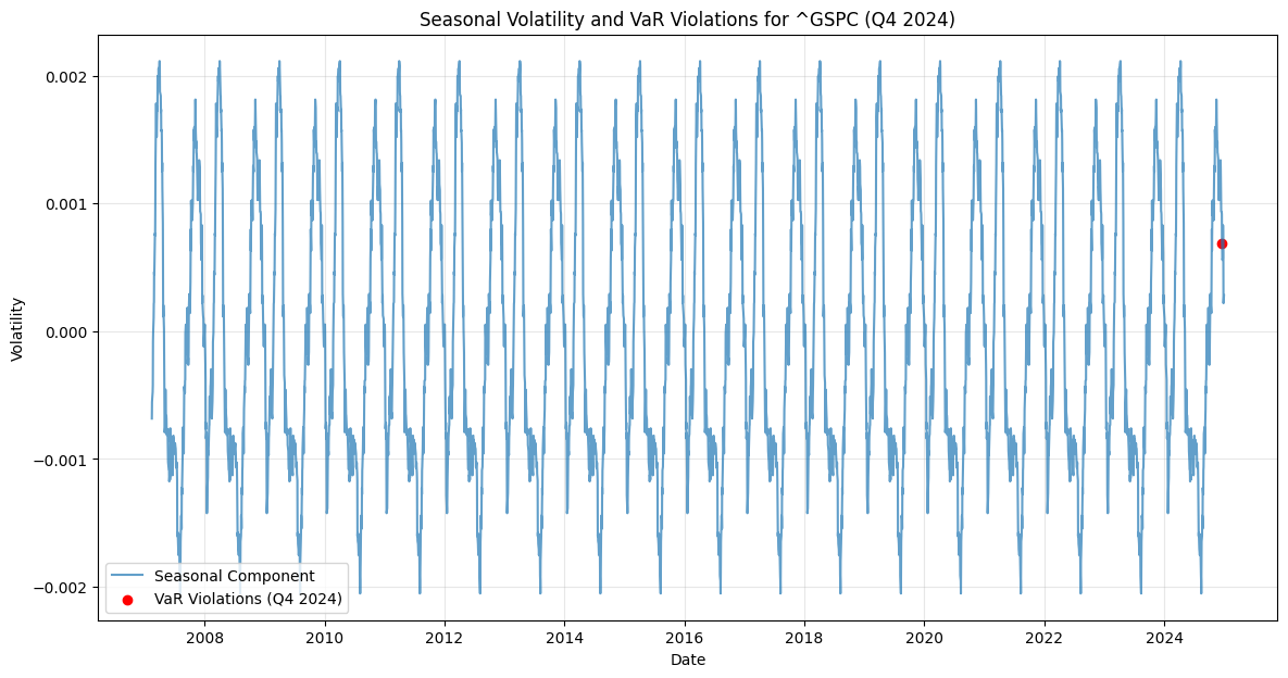
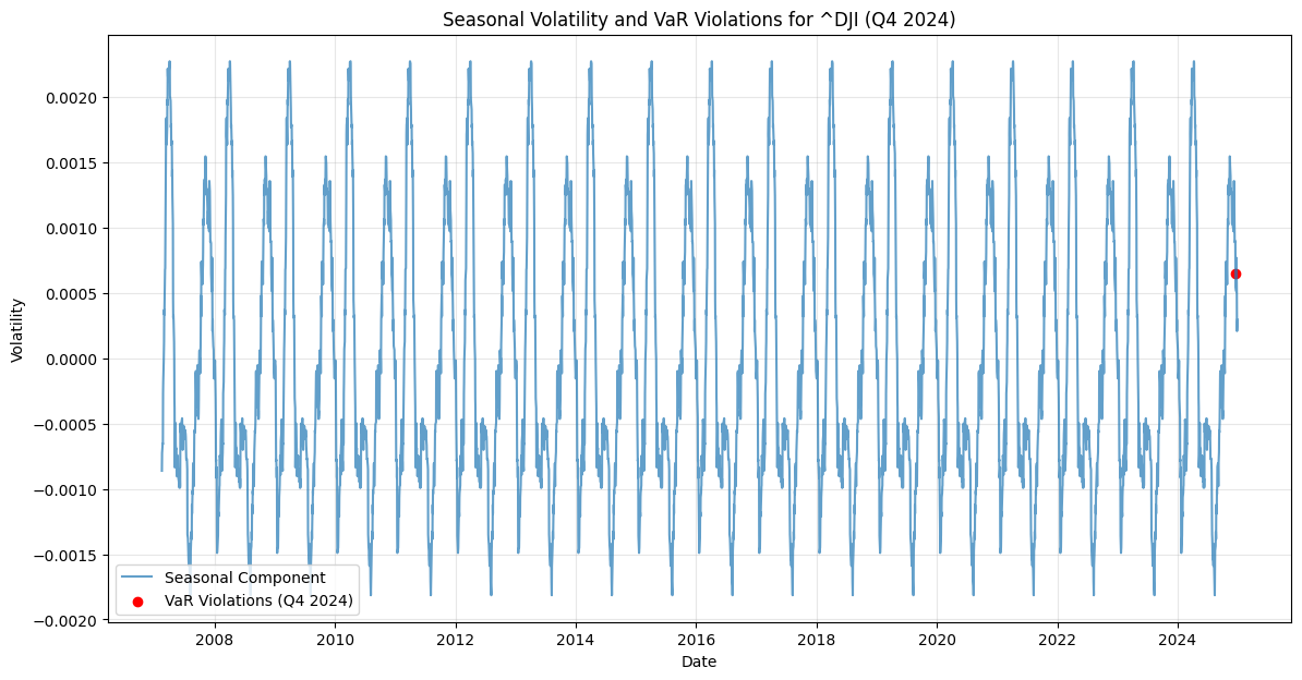
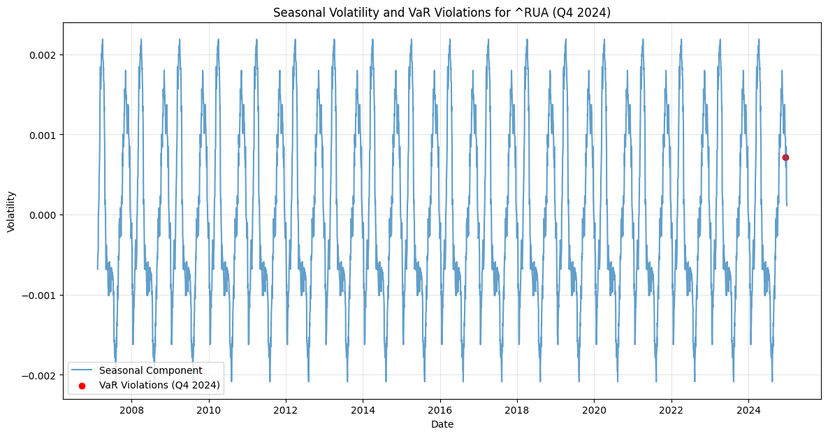
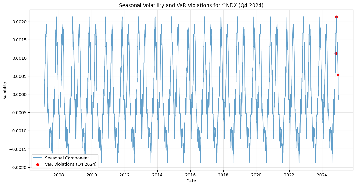
In the charts for ~RUA (Russell 3000 Index) and ~NDX (Nasdaq Composite Index), the seasonal component of volatility is drawn over time. The patterns indicate recurring volatility spikes, likely tied to specific times of the year (e.g., end-of-quarter or year-end effects). For Q1 correction, the seasonal decomposition suggests that volatility may increase in the first quarter due to factors like portfolio rebalancing, earnings reports, and macroeconomic data releases. This insight can help investors anticipate and prepare for potential market adjustments during Q1.In the charts for ~GSPC (S&P 500 Index) and ~DJI (Dow Jones Industrial Average), the seasonal component of volatility also is drawn over time. These patterns reveal recurring volatility spikes, likely associated with events like earnings seasons, macroeconomic data releases, or end-of-quarter portfolio adjustments. For Q1 correction, the seasonal decomposition suggests that volatility may increase in the first quarter due to factors such as January’s portfolio rebalancing, tax-related selling, and the release of annual financial reports. This insight can help investors anticipate and prepare for potential market adjustments during Q1.

